This is a followup to my previous article describing how to compile a hardware accelerated version of OpenCV. You can find that article here, but to briefly recap: part of the Sparkfun AVC is finding and popping red balloons. We wanted to do this using on-board vision processing. For performance reasons we need to hardware accelerate the vision system. We are using the Jetson TK1 board from NVIDIA with the OpenCV library.
What follows is a description of the vision system we developed. The full code for the vision system can be found on github at https://github.com/aiverson/BitwiseAVCBalloons
The OpenCV Project
The Open Computer Vision project (OpenCV) is easy to use and allows you to quickly program solutions to a wide variety of computer vision problems. Normally, the structure of a simple computer vision program using OpenCV is:- read in a frame from a video camera or a video file
- use image transformations to maximize the visibility of the target
- extract target geometry
- filter and output information about the target.
For hardware accelerated applications, OpenCV provides hardware accelerated replacements for most of its regular functions. These functions are located in the gpu namespace which is documented at http://docs.opencv.org/modules/gpu/doc/gpu.html
The Algorithm
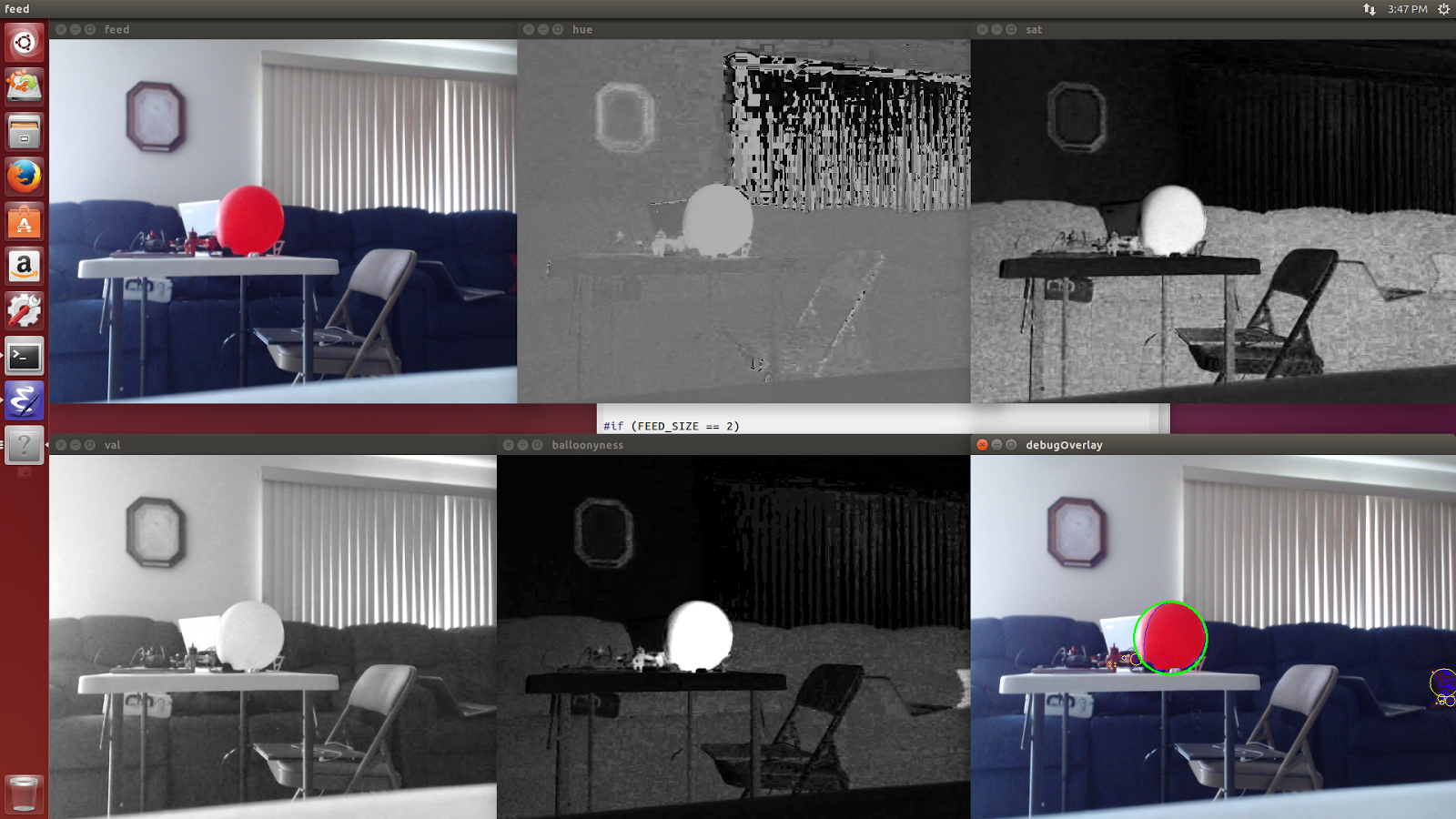
When trying to identify our balloon targets, the first thing I tried was converting the video stream to Grayscale because it is fast and cheap. However, this did not give sufficient distinction between the sky and balloons. I then tried converting the stream to HSV (Hue Saturation Value) because it is good for identifying objects of a particular color and relatively simple to do. The balloons are quite distinct in both the hue and saturation channels, but neither alone is sufficient to clearly distinguish the balloons against both the sky and the trees. To resolve this, I multiplied the two channels together, which yielded good contrast with the background.Here is the code implementing that section of the algorithm.
gpu::absdiff(hue, Scalar(90), huered);
gpu::divide(huered, Scalar(4), scalehuered);
gpu::divide(sat, Scalar(16), scalesat);
gpu::multiply(scalehuered, scalesat, balloonyness);
gpu::threshold(balloonyness, thresh, 200, 255, THRESH_BINARY);
Hue is normally defined with a range of 0..360 (corresponding to a color wheel) but to fit into eight bits, it is rescaled to a range of 0..180. Red corresponds to both edges of the range, so taking the absolute value of the difference between the hue (with a range of 0..180) and 90 gives how close the hue is to red (huered) with a range of 0..90. The redness and saturation are both divided by constants chosen to give them appropriate weightings and so that their product fits the range of the destination. That result, which I call balloonyness (i.e. how much any given pixel looks like the color of the target balloon) is then taken through a binary threshold such that any pixel value above 200 is mapped to 255 and anything else is mapped to zero, storing the resulting binary image in the thresh variable. The threshold function is documented at http://docs.opencv.org/modules/imgproc/doc/miscellaneous_transformations.html#threshold, the GPU version is equivalent.
Once the image has been thresholded, I extract external contours. The external contours correspond to the outlines of the balloons. The balloons are nearly circular, so I find the minimal enclosing circle around the contours. Then, to deal with noise (red things that aren't shaped like balloons), I compare the area of the circle with the area of the contour it encloses to see how circular the contour is.
The image below illustrates this process.
 I could also have used an edge detector and then a Hough circle transform (http://en.wikipedia.org/wiki/Hough_transform) to detect the balloons, but I decided not to because that method would not be able to detect balloons reliably at long range.
The image below illustrates this process.
The Joys of Hardware Acceleration
Before hardware acceleration, this algorithm was running at between two and three frames per second on the Jetson board. With hardware acceleration, it now runs at over ten frames per second, and it is now limited by how quickly frames from the camera can be captured and decoded. This equates to about a five times speedup overall. It is even greater if you only consider the image processing phase.Writing computer vision systems seems very intimidating at first, however there is very good library support so many types of problems can be solved easily with only a little research and experimentation.